Motion planning is one of the biggest problems of current robotics research. From the simple act of controlling a robotic arm all the way to self driving cars, we have yet to find the ideal algorithm for either. However, there are a few core methods for the problem; each of which keeps getting extended to further lengths and applied in various areas. In this post, we shall go through the core ideas, discuss what works, and discuss what doesn’t.
For simplicity, let us consider the case of a robot that can move in any direction, trying to find a way to reach a goal in a 2-dimensional space with some obstacles. Most of the presented algorithms can be extended to more dimensions and other robot types, but need a fair amount of fine-tuning.
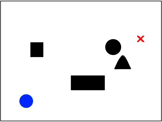
Graph based approaches
The first idea that comes to mind after completing a basic algorithms course is to use algorithms for finding the shortest paths, such as the asymptotically optimal Djisktra’s algorithm. The problem is that the space we are moving in is continuous, while the shortest path graph algorithms require discrete graphs connected with edges.
The most obvious answer is creating a grid that represents the space, treating the points on the grid as vertices, and assigning the edges that lead to an occupied square an infinite cost. On this grid, finding the shortest path is a simple task.
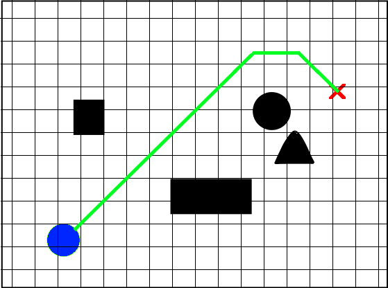
The main problem with this approach is choosing the size and shape of the grid. If the spacing between the vertices is too large, the resulting path diverges further from the optimal one, and the algorithm might not even find a solution in a space with many small obstacles. However, if the spacing is too small, the number of vertices that need to be explored can easily become too large to compute in a reasonable amount of time.
A cleverer method for constructing the graph is to compute a visibility graph. To do so, we need to approximate obstacles with polygons of choice, then, the edges of the polygons become the vertices of our graph. An edge between two vertices exists if there is a straight line unobstructed by obstacles between them, and its cost becomes the euclidean distance between the vertices.
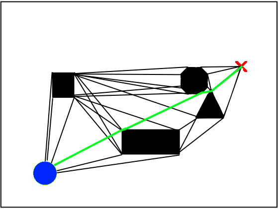
To account for the size of our robot and prevent the algorithm from finding infeasible solutions, we can widen our obstacles by the robot’s radius.
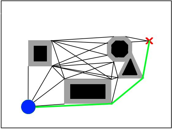
Unfortunately, the method does not scale well to 3 dimensions, as the optimal path rarely leads around obstacles. We also need to be wary of imprecisions in the robot’s movement; a path close to the obstacles could easily lead to a collision upon a mechanical error.
A variation that tries to tackle this is the Voronoi diagram; a graph of points as far away from the surrounding obstacles as possible. This method has led to success in 2-dimensional path planning of mobile robots, but is hard to generalise to 3 dimensions and different types of robots.
Regardless of the resulting shape of the graph, the choice of the shortest path algorithm also matters. Rather than using Djikstra’s algorithm, the more modern approach is the A* algorithm extended with various heuristics. Asymptotically, this algorithm gives us no guarantees, but in practice, it often explores a small subspace of vertices, which can significantly speed up the process of finding the shortest path.
A gradient based approach
Graph based algorithms can give us some guarantees on optimality, but trying to discretize continuous space with high enough precision requires a lot of memory, and searching through the space can easily get too expensive. If we don’t want to search through the whole space and are satisfied with a “good enough” solution instead, we can move away from the graph-based approaches and look for faster algorithms.
One algorithm that stands out is the Artificial Potential Field method. Inspired by physics, each object in the environment acts as a magnet. The target attracts our robot with a strong force, while the obstacles repulse it. In an ideal scenario, this results in finding a smooth path to the target around obstacles.
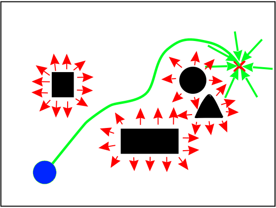
The method is fast and works well in a fair amount of cases, unfortunately, it gives us no guarantees on the optimality of the path. Even worse than that, the method is susceptible to getting stuck in local minima, and not finding a solution at all.
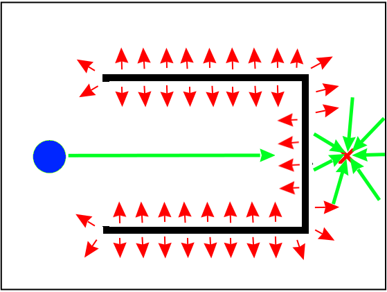
Even so, the algorithm has been used quite successfully, and many extensions that try to combat the local minima problem have been suggested. Some approaches deal with local minima by adding artificial obstacles when the robot gets stuck, while others plan a rough path with a graph based method and use APF to go between the found points.
On state space exploration - a sampling based approach
Arguably the most popular method for motion planning is the Rapidly Exploring Random Tree (RRT) algorithm. The algorithm builds an expanding tree throughout the space, sampling randomly, and creating new vertices until a solution is found.

A solution is usually found quickly compared to the graph based methods, but generally isn’t optimal. The popular variation, RRT*, incrementally improves the found paths whenever possible. Hence, there is a certain trade-off; if we could let the algorithm run infinitely, it would find the shortest path, but since we don’t have infinite time, we need to strike a balance between how quickly we need to find a solution, and how precise it needs to be.
What makes this algorithm popular is its versatility. It’s easy to incorporate constraints, and the state space can easily be extended to further dimensions. The generalisation to 3 dimensions is trivial, but we can go further than that. If we define the state space with respect to the joints of a robot arm, we can sample joint rotations and plan its motion in an environment with obstacles just as easily. Sadly, there is a limit. The size of the state space grows exponentially with each dimension, which makes the algorithm computationally infeasible for limbs with a high number of joints.
Ultimately, there is no clear winner yet. The performance of the respective methods is often comparable in the eyes of a human, hence, the particular choice often depends on the researcher’s familiarity with the algorithm rather than optimality. However, as research keeps pushing further, we keep asking new questions and extending the algorithms further to answer them. Thus, we have yet to see what the motion planning algorithms of the future will be. It could be an extension of the mentioned methods, a new combination of the algorithms, or perhaps something new entirely.
